Overview of ECOSMOS
Contact: Kazuhiro Takemoto (takemoto[at]bio.kyutech.ac.jp).
ECOSMOS reveals community structure of microbial ecosystem; in particular, it estimates cooperative and competitive interspecific interactions from taxonomic composition data (e.g., obtained from 16S rRNA analysis), based on metabolic interactions between microbes.
Displayed Network
The following figure shows an example of ECOSMOS result.
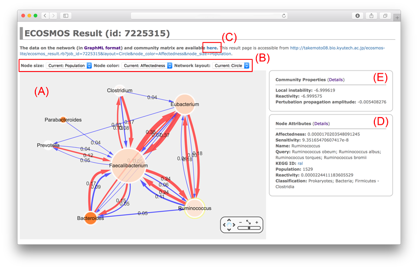
(A) Nodes (◯) and edges (→) correspond to species (taxonomy) and interspecific interactions (cooperation (→) and competition (→)), respectively. Node size and edge weight indicate population and interaction strength, respectively. Note that edges with small weight are removed. In particular, let $w_{ij}$ be the interaction weight between species $i$ and $j$, the displayed network only have edges whose weights satisfy the condition of $$\frac{w_{ij}-\langle w \rangle}{SD}>2,$$ where $\langle w \rangle$ and $SD$ are the average interaction weight and standard deviation, respectively.
You can manually modified the network (e.g., network layout and node deletion).
(B) You can change the options for network drawing.
You can draw the displayed network at your local machine using the GraphML file (job_id)_network.graphml with network visualization softwares such as Cytoscape and igraph. The data are downloadable from (C).
(D) The node/edge attributes are displayed. The details are as follows.
Node Attributes
- Name: taxonomic name on ECOSMOS.
- Classification: the classification category on the KEGG database.
- Population: population of the taxonomic level.
- KEGG ID: KEGG organism ID for species who was used for estimating interspecific (metabolic) interactions.
- Affectedness: how affected nodes are after perturbation propagation.
- Sensitivity: how sensitive nodes are to the initial perturbation.
- Reactivity: perturbation propagation amplitude for nodes.
Edge Attributes
- Interaction type: cooperation or competition
- Weight: interaction weight of a cooperative/competitive interaction
- Related compounds: intermediate metabolites for a cooperative/competitive interaction
Interspecific (Metabolic) Interactions
Interspecific interactions are characterized from genome-scale metabolic networks, obtained from the KEGG (Kyoto Encyclopedia of Genes and Genomes) database. In particular, cooperative and competitive interactions are defined based on the seed score (degree of nutrients), identified using a strongly connected component decomposition algorithm as follows.
A complementary support of nutrients (i.e., cooperation) from species $j$ to species $i$ is defined based the seed scores: $$s_{ij}=\frac{\sum_k \min (S_{i,k}, 1-S_{j,k})}{\sum_k S_{i,k}},$$ where $S_{i,k}$ indicates the seed score of metabolite $k$ in the metabolic networks of organism $i$, and it ranges between 0 and 1 (metabolites with the seed score 0 and 1 indicate products and nutrients, respectively). Note that $s_{ii}=0$.
A scramble for nutrients (i.e., competition) between species $i$ and $j$ for species $j$ is described as $$c_{ij}=\frac{\sum_k \min (S_{i,k},S_{j,k})}{\sum_k S_{i,k}},$$ Note that $c_{ij}$ may not equal to $c_{ji}$ and $c_{ii}=1$.
Interaction Weight
The strength (edge width) of an interspecific interaction of the displayed network is determined as follows. The interaction strength may be also affected by populations; thus, it is defined based on the mass-action law:$$w_{ij}=x_{ij}p_ip_j,$$ where $x_{ij}$ is $s_{ij}$ or $c_{ij}$. $P_i$ is the relative population of $i$, and it is defined as $$p_{i}=\frac{P_i}{\sum_j P_j},$$ where $P_i$ corresponds to the abundance of $i$, estimated using metanogemic analysis.
Dynamic Properties of Microbial Community
ECOSMOS estimates dynamic properties based on random matrix theory [e.g., see (Tang and Allesina, 2014) and (Suweis et al., 2015)]. (E) Specifically, ECOSMOS evaluates the local instability and reactivity of observed ecosystems.
Local Instability
Assuming that the observed state of populations $\boldsymbol{p}=[p_1,\dots,p_n]$ is an equilibrium point, a local stability of an ecosystem is evaluated using the Jacobian matrix $\boldsymbol{J}(\boldsymbol{p})$ under the condition of $\boldsymbol{p}=[p_1,\dots,p_n]$, derived from a Lotka-Volterra system. In ECOSMOS, the following Lotka-Volterra system with $n$ species is considered. In particular, the time evolution $N_i(t)$ of the population size of species $i$ is described as $$\frac{d}{dt}N_i(t)=N_i(t)\left(r_i + \sum_{j=1}^{n}(s_{ji}-c_{ji})N_j(t)\right),$$ where $r_i$ is the growth rate of species $i$.
Assuming that $\boldsymbol{p}$ is an equilibrium point, $r_i$ can be estimated as $r_i = -\sum_{j=1}^n(s_{ji}-c_{ji})p_j$. Since $s_{ii}=0$ and $c_{ii}=1$, the Jacobian matrix $\boldsymbol{J}(\boldsymbol{p})$ at the observed state of populations $\boldsymbol{p}$ is obtained as $$J_{ii}=r_i-2p_i+\sum_{j\neq i}(s_{ji}-c_{ji})p_j=-p_i$$ and $$J_{ij}=(s_{ji}-c_{ji})p_i \mathrm{ \ \ (when \ }i\neq j).$$
The largest real eigenvalue $\lambda_1$ determines local stability of the ecosystem; in particular, negative $\lambda_1$ indicates that the system is locally stable. Moreover, a lower $\lambda_1$ indicates lower local instability of the ecosystem.
Reactivity
The stability analysis based on the largest eigenvalue has a limitation; in particular, it provide no information on the transient response. For example, perturbations may be amplified even if the system is locally stable. The perturbation amplification can be consider in the context of reactivity, defined as the maximum amplification rate over all initial perturbations. In particular, reactivity is evaluated by the largest eigenvalue $\lambda_H$ of $\boldsymbol{H} = \left[\boldsymbol{J}(\boldsymbol{p}) + \boldsymbol{J}(\boldsymbol{p})^T\right] / 2$. For example, the system is locally stable but reactive when $\lambda_1 < 0$ and $\lambda_H > 0$.
Perturbation Propagation Amplitude
The amplitude of the perturbation (asymptotic) propagation (i.e., perturbation propagation amplitude) is measurable as follows: $$\cal{A}_1=\frac{\boldsymbol{u}_1 \cdot \boldsymbol{\xi}}{\boldsymbol{v}_1 \cdot \boldsymbol{u}_1},$$ where $\boldsymbol{u}_1$ and $\boldsymbol{v}_1$ correspond to leading left and right eigenvectors corresponding to $\lambda_1$, respectively. $\boldsymbol{\xi}=(\xi_1,~\xi_2,\dots,~\xi_n)$ indicates a given small perturbation.
In the above example (see figure), the ecosystem (from human gut) is locally stable and it is not reactive. Moreover, the pertubation is not amplified. In short, this indicates that the ecosystem is very stable.
Dynamic Properties for Species
ECOSMOS also evaluate how susceptible species are to perturbations.
The eigenvectors indicate dynamic properties for species; in particular, $\boldsymbol{v}_1$ and $\boldsymbol{u}_1$ correspond to affectedness (i.e., how affected species are after perturbation propagation) and sensitivity (i.e., how sensitive species are to the initial perturbation), respectively. The leading eigenvector $\boldsymbol{w}_H$ corresponding to $\lambda_H$ is reactivity (i.e., perturbation propagation amplitude for species).